Visualizing Frame Dragging in Kerr Spacetime

Importing required modules

import numpy as np

from einsteinpy.geodesic import Nulllike
from einsteinpy.plotting import StaticGeodesicPlotter

Setting up the system

• Initial position & momentum of the test partcle

• Spin of the Kerr Black Hole

• Other solver parameters

Note that, we are working in M-Units (\(G = c = M = 1\)). Also, setting momentum’s \(\phi\)-component to negative, implies an initial retrograde trajectory.

position = [2.5, np.pi / 2, 0.]
momentum = [0., 0., -2.]
a = 0.99
end_lambda = 150.
step_size = 0.0005

Calculating the geodesic, using the Julia back-end

geod = Nulllike(
    position=position,
    momentum=momentum,
    a=a,
    end_lambda=end_lambda,
    step_size=step_size,
    return_cartesian=True,
    julia=True
)

e:\coding\gsoc\github repos\myfork\einsteinpy\src\einsteinpy\geodesic\utils.py:307: RuntimeWarning:

Test particle has reached the Event Horizon.

Plotting the geodesic in 2D

sgpl = StaticGeodesicPlotter(bh_colors=("red", "blue"))
sgpl.plot2D(geod, coordinates=(1, 2), figsize=(10, 10), color="indigo") # Plot X vs Y
sgpl.show()

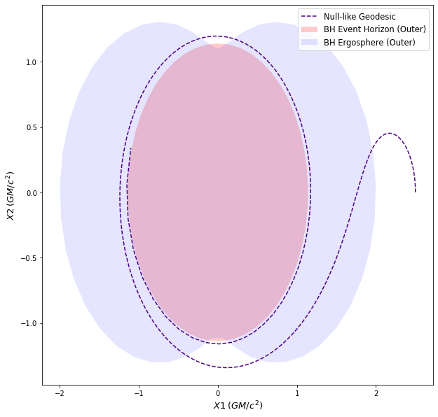
As can be seen in the plot above, the photon’s trajectory is reversed, due to frame-dragging effects, so that, it moves in the direction of the black hole’s spin, before eventually falling into the black hole.